Fast Pathfinding on the dynamic Grid

Problem Definition

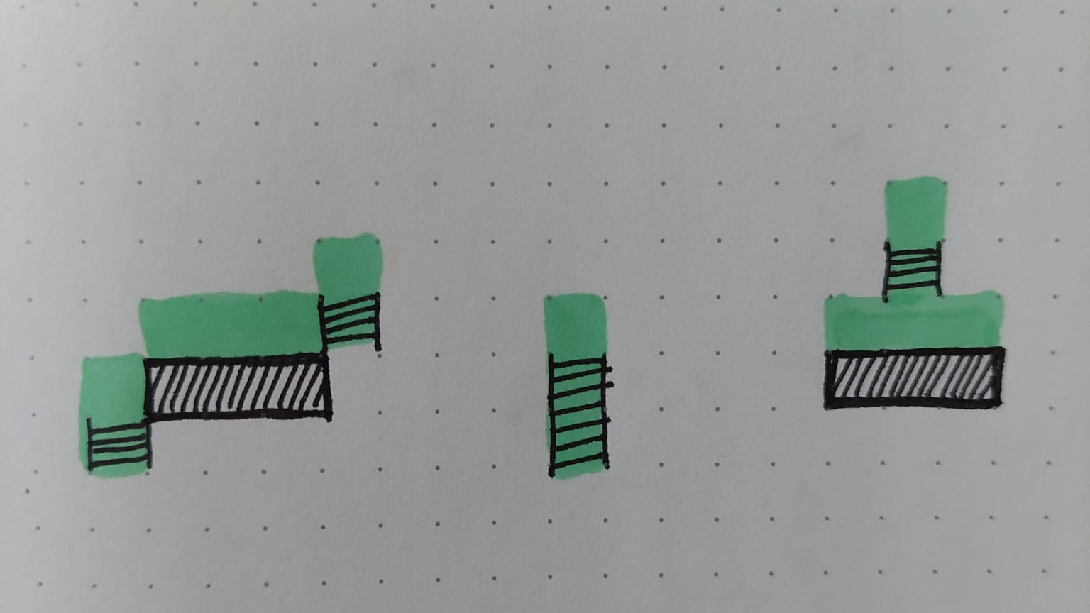
Consider a 2D tile-based game with a side-view perspective. In my case, that game is about worker assignments: The player places tasks anywhere on the map, workers look for reachable tasks to work on.

This makes for an interesting pathfinding problem: During a single simulation frame (“tick”), we may need to compute hundreds of shortest paths, many of which may be unreachable.

We can do some preprocessing at game startup to make this easier, but the map is dynami, so any precomputed information needs to be kept up to date. Since this is not a game about optimal paths, reasonably good paths will do, strict optimality is not required.

This article goes through the implementation I came up with. This is not so much a novel algorithm, merely a writeup of my variation on the ideas in [HAA, HPA, RW] together with some implementation notes.

Before diving into the algorithm, let us briefly define the movement model used throughout the examples:

The game uses side view perspective, characters are of size 1×1 tiles. A characters is considered supported if either:

• it occupies the same tile as a ladder, or
• there is a solid block or a ladder directly beneath it

(Characters can stand on the top sprung of the ladder). Additionally, the tile the character occupies may not be blocked (except for ladders). As long as these conditions are met, characters can move in the 8 directions (top/left/bottom/right + diagonals).

To keep this article digestible, we’ll ignore several complications such as: Clearance (characters being larger than 1×1), Capabilities (flying/swimming units, doors) and Pathfinding Objectives (situations in which the goal is not to move directly onto a tile but close to it).

I’ll occasionaly mentioning Rust crates where relevant, but generally the ideas discussed here are pretty independent of programming language.

A*

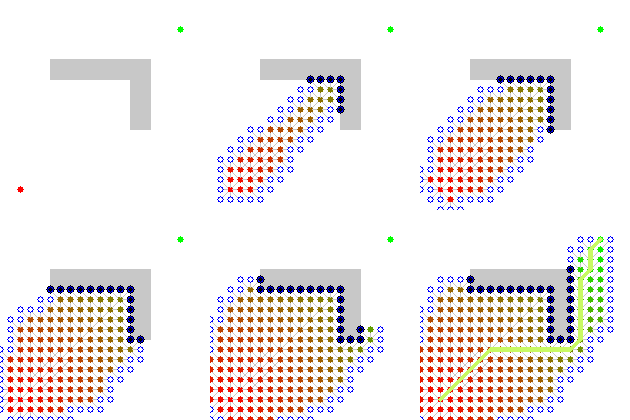
If you have experience with grid pathfinding, you probably heard of the popular A* algorithm [A*]. It uses a heuristic which can greatly speed up pathfinding compared to Dijkstra, in many cases, this makes it extremely efficient in a lot of situations. However, when large obstacles are in the way, this can cause a considerable slowdown. Worse, if the target is unreachable, it explores the ENTIRE reachable map before concluding no path exists.

For a worker-assignment game, this is a serious problem. We may need to evaluate hundreds of potential jobs every frame and its not unlikely that most of them are unreachable.

This leaves us with two goals:

1. Avoid visiting a lot of tiles when there is a big obstacle in the way
2. Have a faster way to determine if there even is a path from source to target.

Building a navigation mesh

In order to tackle these issues we build a Navigation Mesh: A data structure that will maintain navigation information about our map. This servers two purposes:

1. Fast reachability checks – Track which positions are connected at all
2. Hierarchical pathfinding – Compute coarse paths first and refine them later [HAA, HPA, RW]

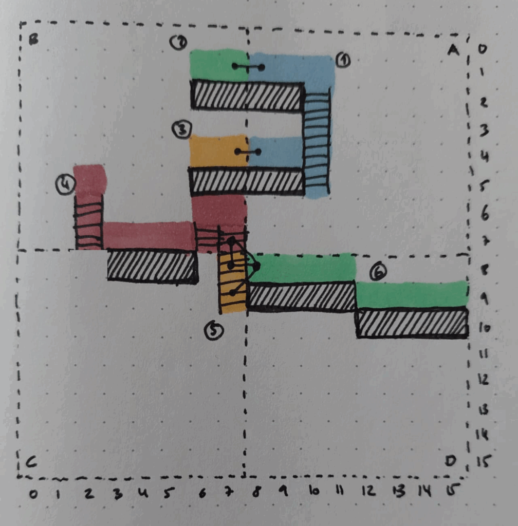
We divide the map into square chunks. Within each chunk, we identify regions: Areas of tiles that are mutually reachable under the movement rules described earlier.

Instead of precomputing shortest paths between every possible entrance and exit point ([HAA, HPA]), I found it more practical to compute only the connectivity information (as is done in [RW]), as the performance of fully precomputing paths did not scale well.

Instead we find regions which are the connected components of the tile graph. Perfomant implementations for connected component computation already exist, for example in [PF]. We know that a path between any two points within such a region can be found by definition, but we’ll compute the actual path only when we actually need it.

Regions are always constrained to their parent chunk. If across a chunk boundary is possible, we connect the corresponding regions with a logical edge denoting the connecting tile positions. In the example above (among others) region (5) in chunk C which connects upward to region (4) in chunk B and to the right to region (6) in chunk D. Visualizing these edges produces the region graph:

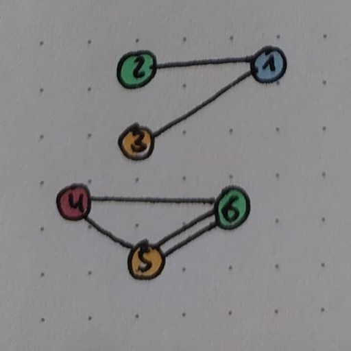
In this graph, each node represents a region and each edge describes a way to get from one region to the other (they may be connected at multiple tiles as is the case for (5) and (6)). We will later see a different way to interpret this graph. Once this graph is built, we compute its connected components.

These connected components give us a global understanding of reachability: A character anywhere in regions 1, 2, 3 can reach any other point in these regions but not any point in 4, 5 or 6. Each region stores the ID of the connected component it belongs to. This will make later reachability lookups extremely efficient at the cost of some maintenance.

Initial Computation

A nice property this setup is that regions can be computed independently for each chunk.

At game startup we process all chunks in parallel. In Rust, this is almost trivial when no shared mutable state is involved, for example using par_iter [PI].

For each chunk, we compute tile connectivity according to the movement rules described earlier, with one improtant restriction: chunk boundaries are temporarily treated as impassable. Then, we find the connected components to identify the chunk’s regions. During this step, we also maintain a chunk-sized tile map of region IDs, allowing constant-time lookup of a tile’s region later.

After all chunks have been processed, we scan chunk boundaries and create inter-chunk edges in the region graph wherever traversal is possible. Each edge stores:

• the two regions it connects, and
• the corresponding boundary tile positions.

Finally, we compute the connected components of the region graph itself and assign each region its global component ID.

Querying Reachability

This is where all the hard work of the preprocessing finally pays off.

In gameplay, we may need to evaluate hundreds of possible jobs in short time, many of which may be unreachable, so reachability checks need to be cheap. Given source and target position, the process is straightforward:

1. Find the region of the source position (find its chunk, check its region tilemap)
2. Find the region of the target position (same process)
3. If both positions are in the same region, the target is reachable.
4. Otherwise, compare their component IDs, if those match, the target must be reachable, otherwise it is not.

Thats all there is to it. Thanks to careful preprocessing, we can determine if there is a path between any two positions on the map (no matter how far apart) with a small constant number of lookup operations.

Pathfinding

Pathfinding is similar, but needs a bit more preparation. Taking a look at our region graph, we have regions that are connected via edges. Those edges contain the two neighboring positions where two regions at a chunk boundary touch. In order to obtain an (approximate) shortest path between two map positions we first compute a shortest path on that region graph and then later refine that.

When computing a path on the region graph we would like to still make use of the efficient A*. However for its heuristic we need to estimate the remaining distance to the target. But remaining distance from where? A region can be relatively large, if we just take any point of the region as reference we might needlessly pessimise the quality of this coarse path.

Instead, we will use the region graph a bit different: Above we viewed regions as nodes and the 1-step touch points between them as edges. This view we now flip on its head: We now view the map positions (we stored in the region graphs edges) as nodes and the regions we interpret as sets of edges (a complete subgraph) between all the map positions they contain. In addition to these edges obtained by regions our new graph also still has the edges of the region graph between two neighboring map positions at chunk boundaries.

Note that this “new graph” is nothing we need to explicitely construct in memory, it is just a different view on the region graph we already have. This view allows us now to apply A* in a straight-forward way: Our nodes are map positions, so remaining distance can be estimated (admissibly) by beeline distance.

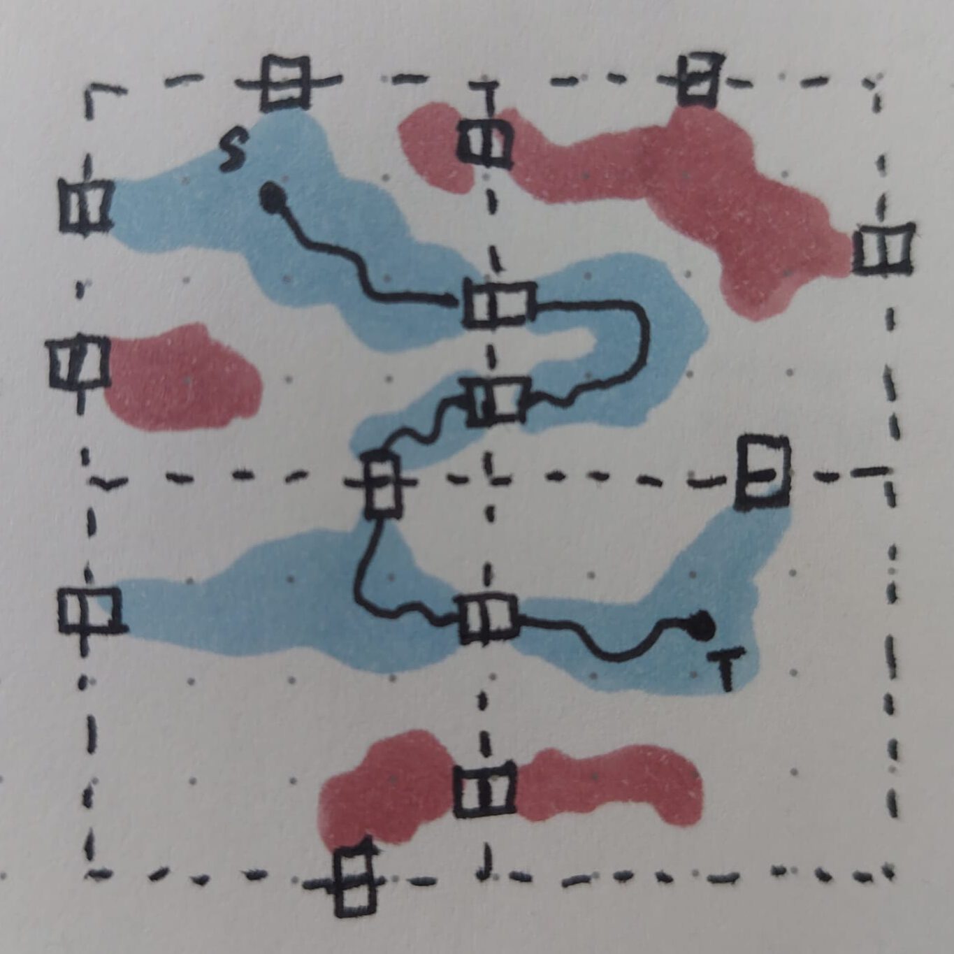
The procedure is as follows:

1. Identify the regions of the source- and target positions respectively
2. Utilize the region graph with map positions as nodes and edges from regions and region-connections as described above
3. From this graph we create an augmented view that also contains the source and target positions, connected to all the other positions their regions are connected to. We track for each logical edge which region it belongs to.
4. On the augmented view, compute the shortest path from the source to the target and record all the nodes and map positions of that shortest path. We may think of this as a sequence (source position, region, position, position, region, position, position, region, ..., region, target position). Map positions other that source and target come in pairs as they are found on the chunk boundaries where they are connected directly to a next position. Note in this view each region is always sandwiched between two map positions.
5. For each region in the found path, compute the shortest path from the previous “entry” map position to the next “exit” position. This computation only ever needs to consider positions inside that region. When done, stitch all the found paths and positions together to obtain the final path

Chunk Recomputation

Finally we have to discuss what to do when the map changes and our regions and connected components become invalidated. First of all, we only react to changes that actually influence navigation: If a block gets replaced by a different kind of block that has the same effect on walkability, there is no point in triggering any sort of update.

If a tile has influence on navigation however, note it may infuence navigation in a different chunk. Eg if we remove the block at (8, 4) in chunk C in the figure above, this actually splits region (4) in chunk B above. With ladders, a single tile change can actually invalidate the navmesh in two chunks at once.

Once we have identified all chunks that need updating, we process each one as follows:

1. Remove all its regions and edges from the region graph and chunk internal datastructures.
2. Recompute the regions as we did in initial construction and compute temporary chunk-internal connected components
3. Connect the chunks regions to regions outside the chunk (scan the chunk boundary for connection points).
4. Carefully repair the connected components: Propagate connected components from outside the chunk inwards along the region graph, match them up with its temporary internal components. If there is a union (two different outside components assigned to a single inside one), we need to walk the region graph and substitute the smaller component with the larger one. If two outside regions with the same component are not joined by this chunk, we need to verify that they are still connected by finding a path in the region graph that does not involve our recomputed chunk. If they aren’t, that component needs to be split (the smaller half gets substituted with a new component id).

This part is much harder to parallelize, but unless your map changes in many different places at once, this is likely not necessary anyway.

And that’s it! Now you have a fast navmesh that can react to map changes, compute fast approximate shortest paths and very fast connectivity checks, congratulations!

Possible extensions include thinking about capabilities (swimming, flying) and clearance (characters of different sizes). If you want to tune the performance some more for very large maps you can take the “hierarchical” i in the “Hierarchical Annotated A*” a bit more serious and build a tree in which chunks in turn are chunked. This however not only makes the code more complex and harder to maintain but also has its own computational overhead so I would advise to first play around with chunk sizes and other tunings before investing into that. In my case path computation on a 1024×1024 map on a couple years old gaming laptop is still nice and fast.

Bibliography

[A*] Wikipedia A* Search Algorithm ( https://en.wikipedia.org/wiki/A*_search_algorithm )
[HPA] Article Clearance-based Pathfinding and Hierarchical Annotated A* Search ( https://web.archive.org/web/20190411040123/http://aigamedev.com/open/article/clearance-based-pathfinding/ )
[HAA] Paper Hierarchical Path Planning for Multi-Size Agents in Heterogeneous Environments ( https://web.archive.org/web/20180723170739/https://harablog.files.wordpress.com/2009/01/haa.pdf )
[RW] Youtube RimWorld Technology – Region System https://youtu.be/RMBQn_sg7DA?si=ei5y0xemjTZEWpug
[PF] Crate Pathfinding ( https://docs.rs/pathfinding/latest/pathfinding/ )
[PI] Crate Rayon: par_iter ( https://docs.rs/rayon/latest/rayon/iter/index.html )