Spatial Hashing vs ECS

We consider an issue that appears frequently in game development and simulation projects: We have many moving points in a 2d world and need to find out which points are in range of which other points. We’ll call this the “range query problem” here (even though that is a bit imprecise). This has several applications:

• Detecting collisions of units (either directly or as a preprocessing step before doing more complex polygon intersection operations)
• Figuring out which units are affected by weapons range or areal effects.
• Detecting partners for chemical or other interactions in simulations, perhaps also useful for simplifying simulation of gravity effects

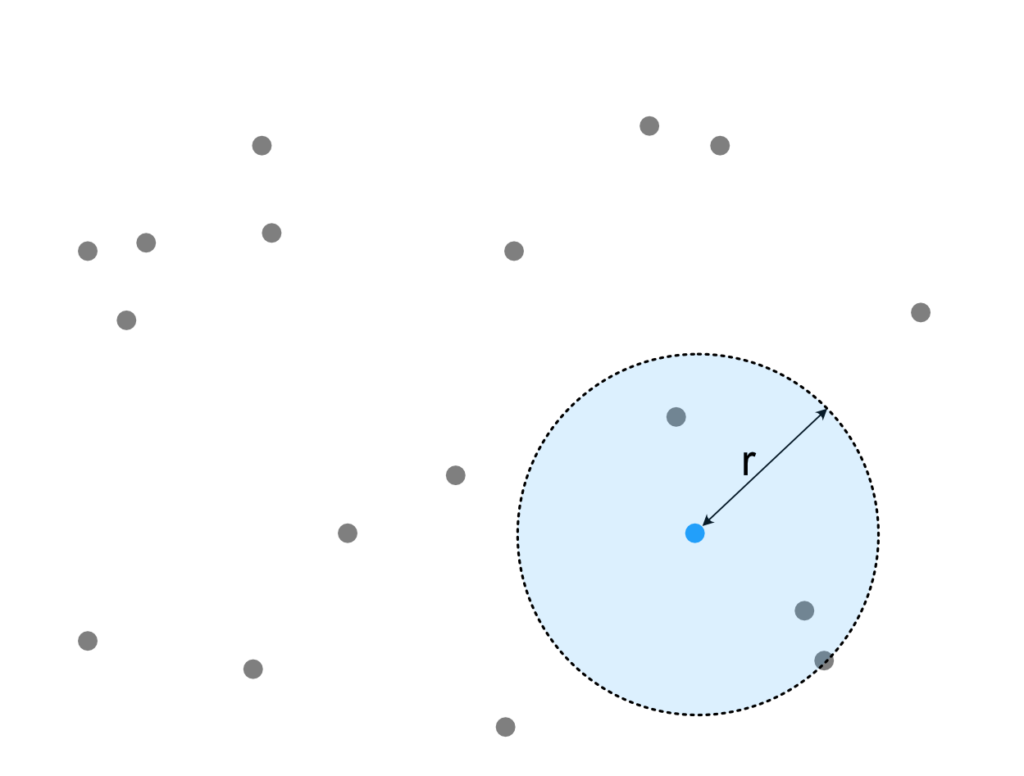
The techniques discussed here easily extend to any number of dimensions (curse of dimensionality may apply though), but for this discussion we’ll focus on the 2d case. Some of the discussed methods (in particular Spatial Hashing) extend easily to arbitrary shapes but for simplicity we’ll stick to circular or square radii. Figure 1 illustrates the situations: Many points are on the plane and we are interested in the points inside the query area (blue dashed circle) which is centered around the query point (blue point).

We’ll briefly introduce how you would address this issue in the most straightforward way in any Entity Component System (ECS), briefly touch on the pros and cons of tree-based methods and then dive a bit into Spatial Hashing and how one could implement such a thing in Rust (for use in Bevy in particular). In the end we’ll spend some time comparing the ECS approach and Spatial Hashing in terms of performance to provide some intuition on when it might be worth it to use one over the other and what good parameter ranges could be.

ECS / “Flat” Approach

An Entity Component System or “ECS” for short is a design pattern that comes in handy in game development, when you have to deal with a lot of objects (Entities), each of which has some subset of a range of properties (Components). I.e. some can move, some can be drawn to the screen, some have a health bar, some can be selected by the user, etc…). If a lot of different combinations of these exists among your objects, a class hierarchy might just not be the best approach to express this. An ECS approach can help in that case.

ECS’s do a lot of useful things that I wont get into in the scope of this post (there should be plenty of resources about it on the net), but one thing that I do like to mention is that they will typically story data about their entities in a very specific way: Instead of packing all data together with the entity in a struct or class like so:

struct Entity {
  position: Optional<Vec2>; // Not all entities have a position
  name: Optional<String>; // ... or a name ...
  animation: Optional<ImageHandle>;

  // ... whatever other components you may think of ...
}

Instead of such a vector of entity objects, ECSs will do something more similar to the code below. That is, it will store the same kind of component from the different entities together:

type Entity = u32;

struct Entities {
  positions: Vec<Optional<Vec2>>,
  names: Vec<Optional<String>>,
  animation: Vec<Optional<ImageHandle>>,
  
  // ... whatever other components you may think of ...
}

This allows very performant access if you work with only a few components, but want to touch most or all of the entities that have them (this is what the Systems in ECS do). I.e. for each entity you want to read its speed vector and update its position from it. This would require iteration along only two vectors which is both space efficient and sequential and thus very cache friendly. And it turns out, caches these days are so fast that for many practical problems they are more important than asymptotic complexity [citation missing].

This is still a blatant oversimplification on how ECSs store their data, in reality its much more clever (see for example https://docs.unity3d.com/Packages/com.unity.entities@0.1/manual/ecs_core.html on Archetypes), for our discussion here it is enough to understand that all the positions of our objects will be tightly packed in memory and thus an exhaustive scan will be rather efficient. Using this directly for spatial range queries is betting everything on efficient caching mechanisms at the cost of completely ignoring asymptotic complexity. Or to put it even simpler: We gladly do way too many operations but thanks to caching they will also be super fast.

We already mentioned it above; the ECS we’ll be using here (for both the “ECS approach” and as a basis for Spatial Hashing) is Bevy.

Spatial Tree Structures

A common approach to spatial data structures is to form some sort of tree such as a K-D-Tree (in our case with K=2), Quad-Tree, R-Tree, etc… (the list is virtually infinite). Since I’m trying to argue about a rather large class of data structures here in one go, this is gonna be very hand-wavy, but I hope I can convey you a gut feeling.

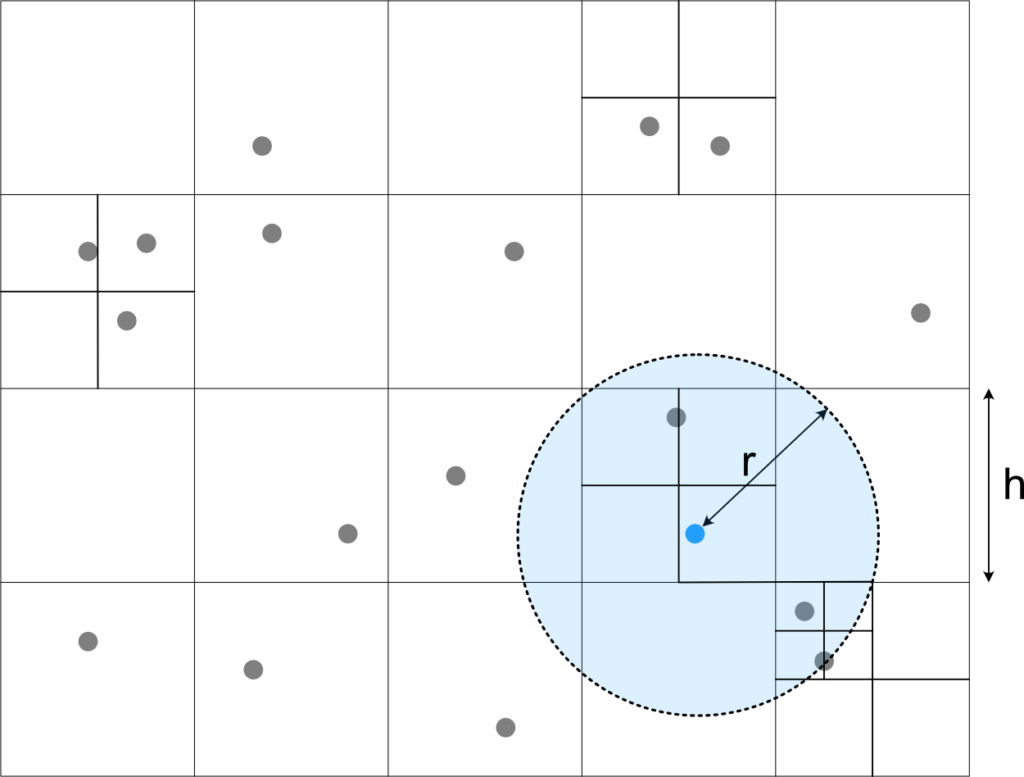
The general idea is usually the same: You partition the space in some simple way, say by splitting it in half (for some definition of half \(\rightarrow\) that’s a K-D-Tree) or into quadrants (Quadtree), then you repeat for each part until the resulting spaces are “small enough”. The result then looks something like Fig. 2, i.e. the data structure is more fine-grained where the points are denser and coarser where there are only little points. This then gives you something like a \(\Theta (\log n)\) insert/update/lookup and also rather efficient range queries.

The big strength for these class of data structures is their flexibility: You don’t need to know anything about the distribution of your points or what ranges your queries will be; a tree structure will usually adapt very nicely to whatever you have. There is two downsides to this: Your data access will usually not be very sequential so this is not cache-friendly in the common case, the other is maintaining & navigating these structure costs time: Most of the operations will be \(\Theta (\log n)\). This will often hold even if you’re updating a point that you know everything about that there is to know, which in the ECS case would cost no more than \(\Theta (1)\).

Grid Methods (eg Spatial Hashing)

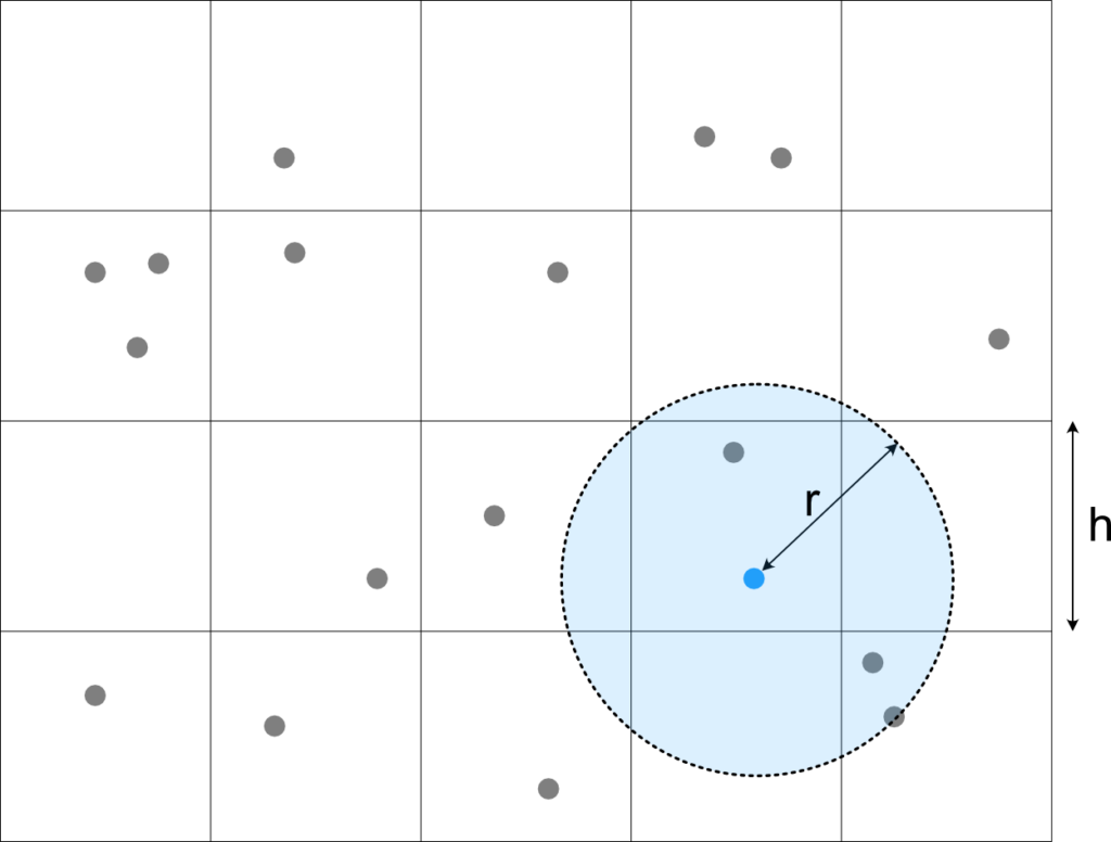
Grid methods simplify the idea of tree-based methods in the sense, that they sometimes can be considered a single layer of a spatial tree. In general, we divide our space (in our case 2d) into square cells of size \(h \times h\) and then have some efficient ways of figuring out a) which cells we need to consider and b) to keep track of what is in each cell. Plenty variants of this pattern exist and it seems the nomenclature is much less well defined than for tree structures. We’ll just give one definition here so we have something to talk about, but just be aware this is not the only way to do it (in particular wrt the choice of data structures being used).

We assume here each point has some sort of ID which we’ll call Entity or EntityID. Each cell is represented as Cell = HashMap<Entity, Position> that lets us quickly check whether an Entity is in the cell and where exactly it is. If we want to find specific points in the cell, we can just iterate the whole hashmap (\(\Theta (n)\)) and a known entity can be removed in \(\Theta (1)\).

Cells themselves are managed in a HashMap<CellIndex, Cell> that maps the integer cell coordinate (eg. (4, 7)) to the cell contents (if the cell contains anything at all).

Figure 3 illustrates how this can be used for fast queries: We first identify the cells which overlap with the query area (here any cell that has part of the blue circle) and then scan each cell for all points that are precisely in the area (by iterating through the HashMap<Entity, Position>. It should be apparent that this needs to check way fewer points than the ECS method above so has the potential of being much faster. This saving however comes at some maintenance cost: Whenever an entity moves, we need to check whether it has crossed a cell boundary. If so, we need to remove it from one cells hash map and put it into the next one.

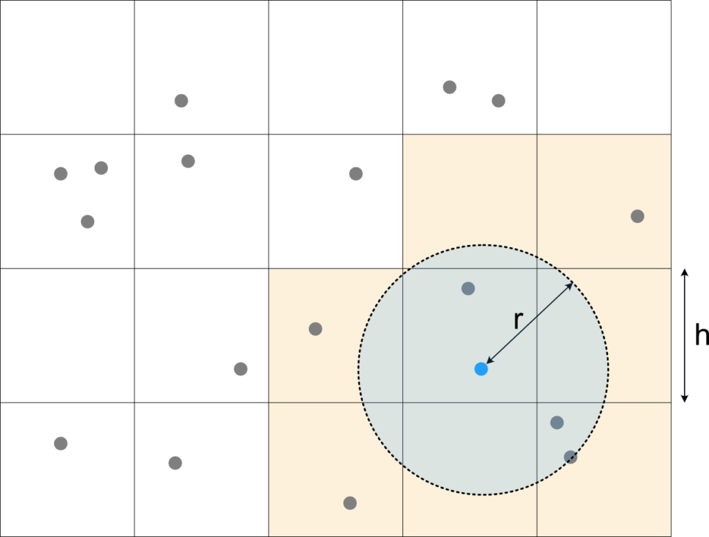
It is worthwhile to note that the choice of \(h\) here should be dependent or \(r\), which implies that wildly changing query radii can not efficiently be supported with a single Spatial Hashmap. In the interwebz I found recommendations like setting eg \(h=2r\). Which intuitively makes sense: In this case we would never need to query more than 9 cells (see eg Fig. 4 where 8 need to be queried). This is not necessarily optimal though, as it depends on the relative cost of accessing a more cells (small \(h\)) vs scanning extra points because of too large cells (large \(h\)). We’ll know at least a bit more at the end of the comparison chapter below.

Further Reading

• “SimonDev” video on spatial hashing in JS. In this variant, points have a size so can be in multiple cells at once.
• “10 Minute Physics” video on a compact spatial hashing implementation.

Rust Implementation

The basic data structures are SpatialHashmap, and Grid. The latter holds the chosen grid spacing together with some simple methods to convert between coordinates and cell indices which we shall skip here (full code will be attached below). The SpatialHashmap also holds a hash map attribute which maps a 2d grid position (IVec2) to a second hash map which maps an Entity to its precise position (Vec2).

#[derive(Debug)]
pub struct SpatialHashmap {
    pub grid: Grid,
    hashmap: HashMap<IVec2, HashMap<Entity, Vec2>>,
}

#[derive(Debug, Clone, Copy)]
pub struct Grid {
  pub spacing: f32,
}

Inserting an Entity into the hash map is straight forward: Compute the relevant grid cell and insert the entity together with its position into the nested hash map. In case that nested hash map does not exist yet (because the cell was so far unused), create one (that’s done by the or_insert(...) part).

pub fn insert(&mut self, position: Vec2, entity: Entity) {
    let index = self.grid.index2d(position);
    self.hashmap
        .entry(index)
        .or_insert(default())
        .insert(entity, position);
}

Updating is only slightly more involved. In case the entity moved across a cell boundary, we need to remove it from the old cell and insert it into the new one, otherwise, updating the position of the entity in its cell is enough:

pub fn update(&mut self, entity: Entity, previous_position: Vec2, new_position: Vec2) {
    let prev_index = self.grid.index2d(previous_position);
    let new_index = self.grid.index2d(new_position);

    if new_index != prev_index {
        // If old cell exists, remove entry from it
        self.hashmap.entry(prev_index).and_modify(|h| { h.remove(&entity); });
    }

    // Ensure new cell exists and insert entity into it
    self.hashmap.entry(new_index)
        .or_default()
        .insert(entity, new_position);

}

In principle we want to allow different kinds of range query type: You might be interested in the square around the query point or the circle or some other weird shape (e.g. your collision polygon). This we encode with the Query trait:

pub trait Query: Debug {
    fn first_cell(&self, grid: Grid) -> IVec2;
    fn next_cell(&self, cell: IVec2, grid: Grid) -> Option<IVec2>;
    fn in_range(&self, position: Vec2) -> bool;
}

The implementing struct will hold the query position and whatever extra parameters (eg radius) it needs and tell us:

• The first grid cell to search (first_cell)
• How to find the next cell to investigate from a given cell, and when to stop (next_cell)
• And, for any precise position, whether it is considered within range or not.

For doing our actual range query, we iterate over all candidate cells with first_cell and next_cell and check each entity in these cells with in_range. The perhaps most straight forward solution here would be to allocate a vector and fill it with all those found entities. However we expect this code to be rather performance critical and are trying to beat a highly cache optimized ECS implementation so we avoid the memory allocation here and define our own Iterator:

pub struct SpatialHashmapIterator<'a, Q: Query> {
    query: Q,
    current_cell: IVec2,
    entity_iterator: Option<hash_map::Iter<'a, Entity, Vec2>>,
    shm: &'a HashMap<IVec2, HashMap<Entity, Vec2>>,
    grid: Grid,
}


impl<'a, Q> Iterator for SpatialHashmapIterator<'a, Q> where Q: Query {
    type Item = (Entity, Vec2);

    fn next(&mut self) -> Option<Self::Item> {

        // If we have an entity iterator (i.e. we are in a valid cell),
        // iterate until we find an entity that is in range or the iterator is exhausted.

        if let Some(mut it) = self.entity_iterator.take() {
            while let Some((&entity, &pos)) = it.next() {
                if self.query.in_range(pos) {
                    // put back the iterator for next time
                    self.entity_iterator = Some(it);
                    return Some((entity, pos));
                }
            }

            // No point in putting back an exhausted iterator
            //self.entity_iterator = Some(it);
        }

        // Is there a next cell we should be looking at?
        while let Some(next_cell) = self.query.next_cell(self.current_cell, self.grid) {
            self.current_cell = next_cell;
            if let Some(entities) = self.shm.get(&self.current_cell) {
                self.entity_iterator = Some(entities.iter());
                return self.next();
            }
        }

        // No cells left to check, we have seen it all!
        None
    }
}

Source Code

Its not quite something I would dare publish on crates.io yet, but if you are curious, you can find the full source code (including the plotting scripts for the comparison below) at https://github.com/Droggelbecher/bevy-spatial-hashing .

Comparison

Asymptotic Complexity

Method	Insert	Update	Query
ECS	\(\Theta(1)\) amortized	\(\Theta(1)\)	\(\Theta(n)\) but very cache local
2-D-Tree [wp]	\(\Theta(\log n)\) on average	\(\Theta(\log n)\) on average	\(\mathcal{O}(\sqrt{n} + k)\) worst case
Spatial Hashing	\(\Theta(1)\) amortized	\(\Theta(1)\) amortized	\(\Theta(k + r^2 \cdot d)\) \(\approx \Theta(k)\) for \(r = const.\) and homogeneous density \(d\)

Table 1 shows a quick overview of the asymptotic complexities of some approaches. For ECS we assume basically a flat vector with entity coordinates and some \(\mathcal{O(1)}\) mechanism to get vector indices from entity IDs, so the costs boil down to appending to that vector (Insert), updating an element (Update) and scanning the whole vector (Query).

For the K-D-Tree with K=2, Insert and Update are \(\mathcal{O}(\log n)\) on average as it is a self-balancing tree. Query complexity is taken from the linked Wikipedia article. Note that \(k\) here refers to the number of found points and is just there to express that in case \(k \ge \sqrt{n}\), \(k\) would of course dominate the query time.

For Spatial Hashing we assume insert and update of the utilized hash maps to be \(\Theta(1)\) in the average case as is generally the case for hash maps. For Query, we for sure need to iterate through \(k\) found points, visit \(\Theta (r^2)\) grid cells, each containing some \(d\) (for Density) points. We assume on average that the fraction of query area over the area of totally queried cells is constant and thus is the fraction of found points over considered points is, assuming the density is homogeneous on average, thus, for a constant query radius \(r\), this boils down to \(\Theta (k)\).

Test setup

Using Bevy 0.9 we created a simulation of 10000 points uniformly distributed on a rectangular 2000×1000 rectangular area. Points were continuously moving with a uniform random speed chosen from (-10, -10)..(10, 10), “bouncing off” the area boundaries when they touch them. In order to get rendering costs out of the equation, the simulation was completely headless (inspired by Bevy’s headless.rs example). Each frame, for each of the 10k points, all points within a \(2r \times 2r\) square centered around that point were computed with either scanning the ECS or the Spatial Hashing method. For each found point, std::hint::black_box was called in order to prevent the optimizer from discarding the relevant loop code. Spatial Hashing used a configurable grid size \(h\). For reproducibility, the random seed was initialized to a constant at simulation start.

The app was compiled in release mode for the x86_64-pc-windows-gnu target. After one second, the average frame duration was computed and written to stdout together with the simulation parameters and the simulation for this combination of parameters ended. The simulation was run multiple times for different values of the query radius \(r\), the grid size \(h\) and whether or not to use Spatial Hashing.

Analysis

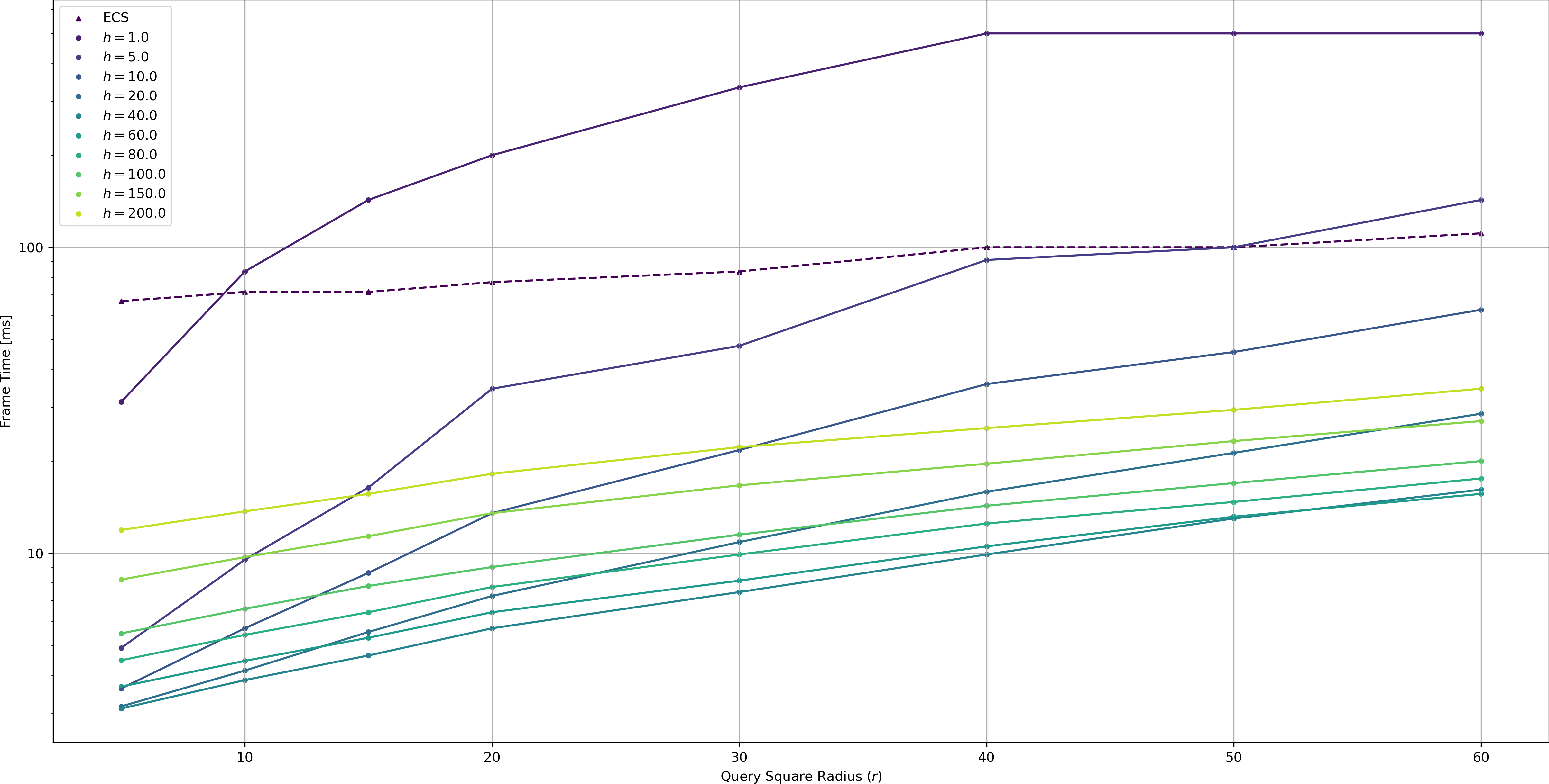
Fig. 6 shows frame times on a logarithmic scale dependent on query square radius \(r\) and grid size \(h\).

With all methods a smaller query square radius leads to faster frame times due to simply fewer points being queried for. The ECS methods performance varies little with query square radius compared to Spatial Hashing. This is to be expected since the number of points to iterate through for this method does not change, but only the number of points processed.

Spatial Hashing in contrast is very dependent on query square radius. For all tested grid sizes, smaller query square radii were smaller. This effect is more pronounced than with the ECS method which is to be expected (there is fewer both fewer cells to check and fewer points to process). Perhaps a bit more surprising is that the optimal grid size for most radii seems to be around \(h=40.0\), rather than eg \(h=2r\). This suggests that in these observations the frame time is not dominated by the query process (which should behave optimal for a certain \(\frac{r}{h}\)), but rather the updating process.

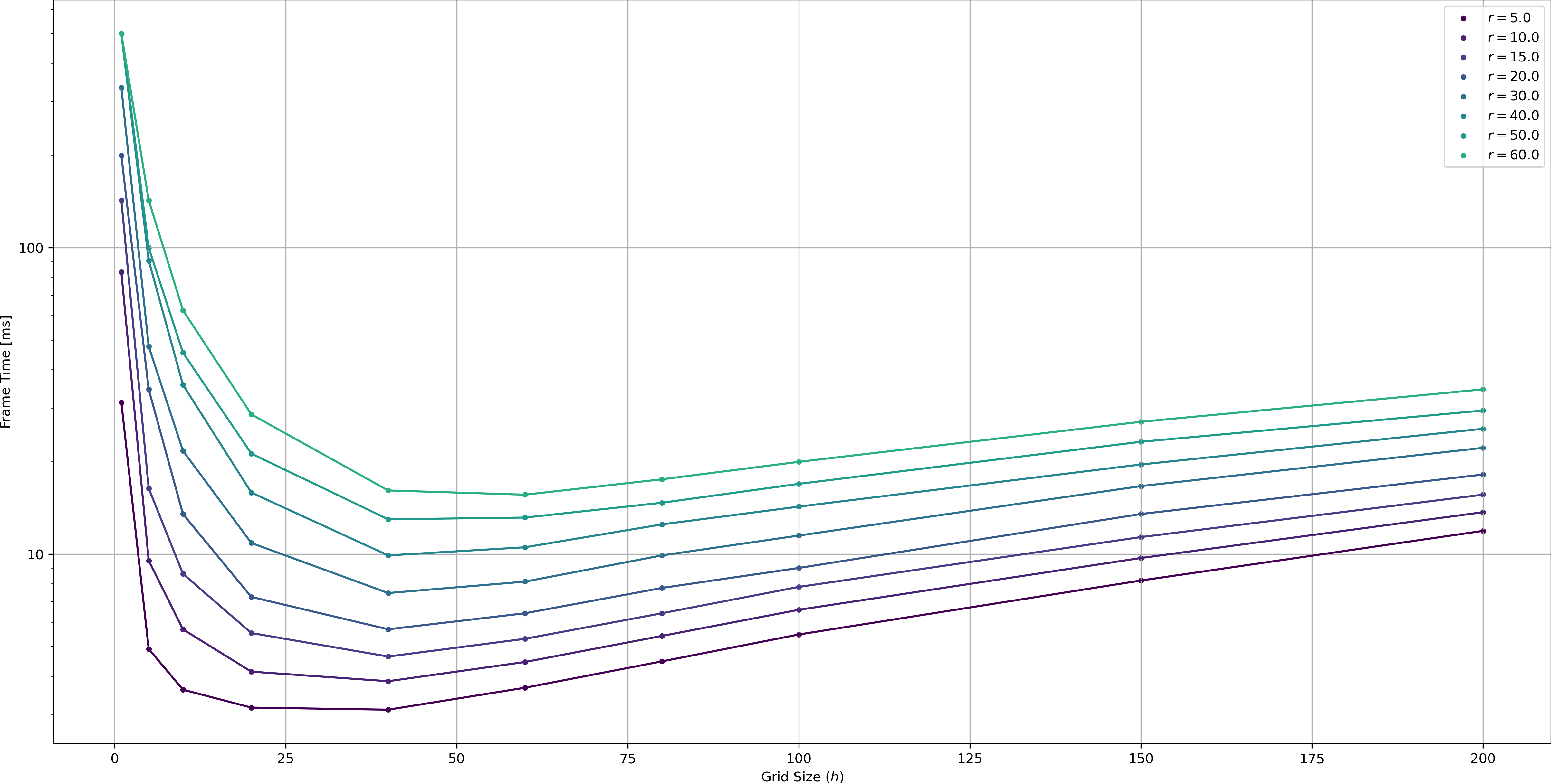
Figure 7 plots the frame time by grid size rather than query radius and sheds some more light on this effect. Points move with an average absolute speed of \(\sqrt{5^2 + 5^2} = \sqrt{2}\cdot 5 \approx 7\), so for grid sizes that are close to (or even below) that value, a lot of points will change cells in every frame which costs a lot of time ¹A detailed probabilistic analysis is left as an exercise for the reader.. Then again for very large grid sizes, we spend more time during querying, as we have to iterate through a lot of points. In this case, for a uniform random speed in (-10, -10)..(10, 10), the sweet spot seems to be around \(h=40\), likely dependent on the point density (lower density mans we can “afford” larger cells as they will contain fewer points).

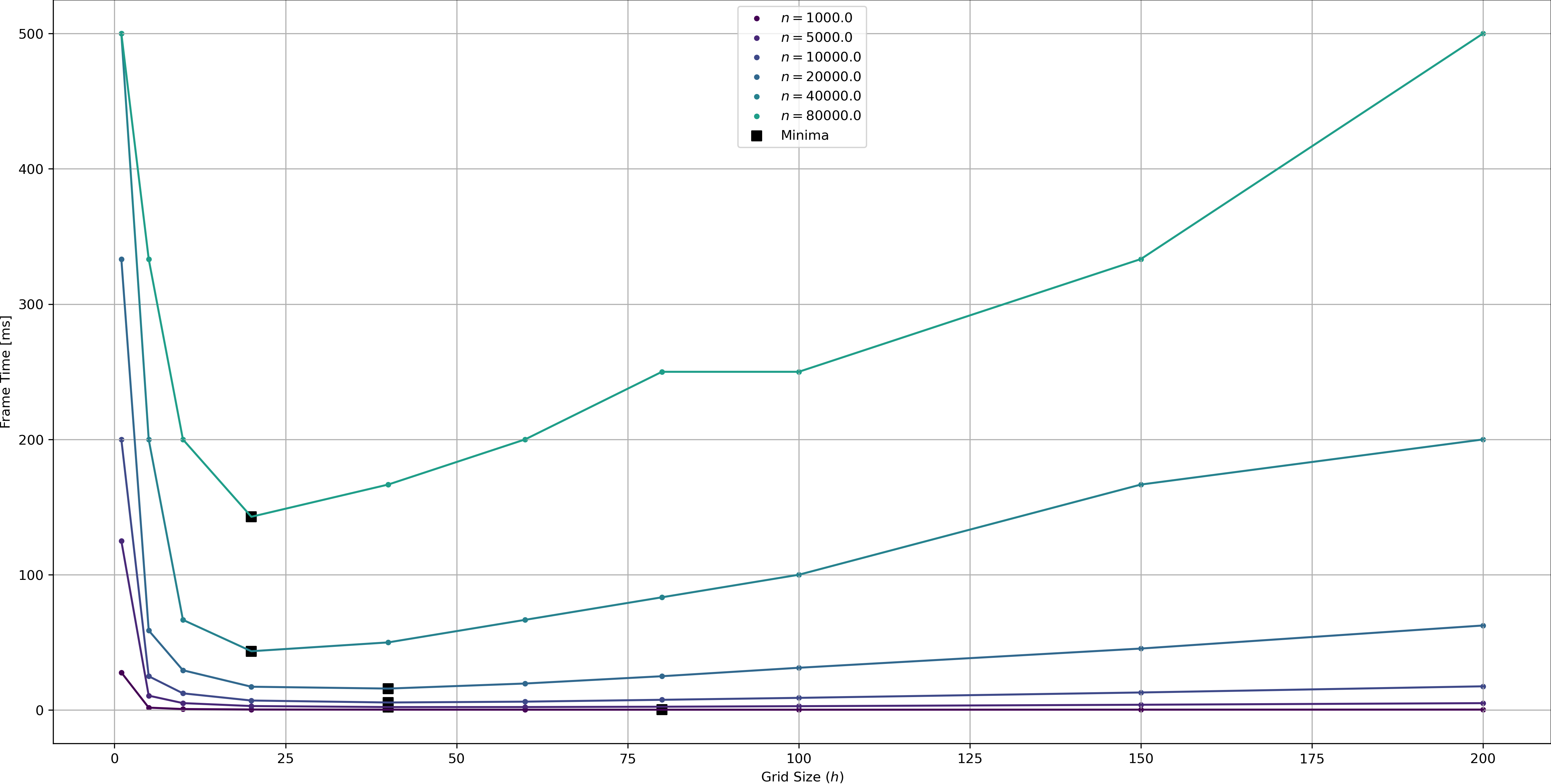
Figure 8 illustrates this effect: Lower densities / point counts lead to larger optimal grid sizes; the effect seems to be relatively weak however (i.e. moving from \(n=10000\) to \(n=80000\) only halves the optimal grid size). Of course in any real game the point distributions and movements speeds will not be this uniform so in practice you’ll have to do your own benchmarks. We can however still collect some takeaways that may transfer to real life to some degree:

• Spatial Hashing can give you a decent speed up over just scanning your ECS, especially when you have a lot of points to query.
• Choosing a good grid size can have a huge impact on performance.
• If you have few points, larger cells are optimal, but also the effect of cell size is not so strong so its ok to choose a too small grid size.
• If you have many (moving) points, the optimum grid size is mostly determined by point speed. Choose your grid size such that points do not cross cell boundaries too frequently, as the slope on the right of Figure 7 is shallow²Unless the query radius is small compared to the average speed, see Fig. 7 for low \(r\)., rather err on the side of a slightly too large grid.